Fall 2025 CS543/ECE549

Assignment 3: Homography stitching

Due date: Mon, October 30, 11:59:59 PM

Contents

• Part 1: Stitching pairs of images
• Grading checklist

1. Download the starter code.
   
   
2. Load both images, convert to double and to grayscale.
   
   
3. Detect feature points in both images. You can use this Harris detector code (it is also copied into the starter .py file), or feel free to use the blob detector you wrote for Assignment 2.
   
   
4. Extract local neighborhoods around every keypoint in both images, and form descriptors simply by "flattening" the pixel values in each neighborhood to one-dimensional vectors. Experiment with different neighborhood sizes to see which one works the best. If you're using your Laplacian detector, use the detected feature scales to define the neighborhood scales.
   
   Alternatively, feel free to experiment with SIFT descriptors. You can use the OpenCV library to extract keypoints and compute descriptors through the function cv2.SIFT_create().detectAndCompute. This tutorial provides details about using SIFT in OpenCV.
   
   
5. Compute distances between every descriptor in one image and every descriptor in the other image. In Python, you can use scipy.spatial.distance.cdist(X,Y,'sqeuclidean') for fast computation of Euclidean distance. If you are not using SIFT descriptors, you should experiment with computing normalized correlation, or Euclidean distance after normalizing all descriptors to have zero mean and unit standard deviation.
   
   
6. Select putative matches based on the matrix of pairwise descriptor distances obtained above. You can select all pairs whose descriptor distances are below a specified threshold, or select the top few hundred descriptor pairs with the smallest pairwise distances.
   
   
7. Implement RANSAC to estimate a homography mapping one image onto the other. Report the number of inliers and the average residual for the inliers (squared distance between the point coordinates in one image and the transformed coordinates of the matching point in the other image). Also, display the locations of inlier matches in both images by using plot_inlier_matches (provided in the starter .ipynb).
   
   A very simple RANSAC implementation is sufficient. Use four matches to initialize the homography in each iteration. You should output a single transformation that gets the most inliers in the course of all the iterations. For the various RANSAC parameters (number of iterations, inlier threshold), play around with a few "reasonable" values and pick the ones that work best. Refer to the alignment and fitting lectures for details on RANSAC.
   
   Homography fitting, as described in the alignment lecture, calls for homogeneous least squares to start a numerical optimizer. The solution to the homogeneous least squares system AX=0 is obtained from the SVD of A by the singular vector corresponding to the smallest singular value. In Python, U, s, V = numpy.linalg.svd(A) performs the singular value decomposition and V[len(V)-1] gives the smallest singular value. I would use SCIPY's scipy.optimize.minmize(see the manual page) to minimize the error in image coordinates.
   
   
8. Warp one image onto the other using the estimated transformation. In Python, use skimage.transform.ProjectiveTransform and skimage.transform.warp.
   
   
9. Create a new image big enough to hold the panorama and composite the two images into it. You can composite by averaging the pixel values where the two images overlap, or by using the pixel values from one of the images. Your result should look something like this:
   
   
   
10. You should create a color panorama by applying the same compositing step to each of the color channels separately (for estimating the transformation, it is sufficient to use grayscale images).

• Extend your homography estimation to work on multiple images. You can use this data, consisting of three sequences consisting of three images each. For the "pier" sequence, sample output can look as follows (although yours may be different if you choose a different order of transformations):
  
  
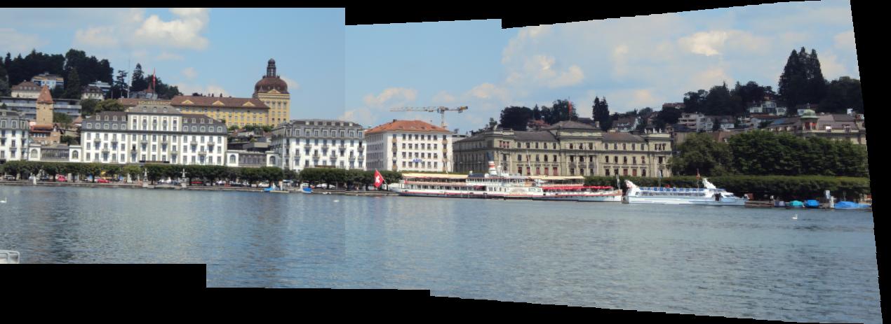
  Alternatively, feel free to acquire your own images and stitch them.
  
  
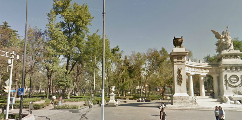
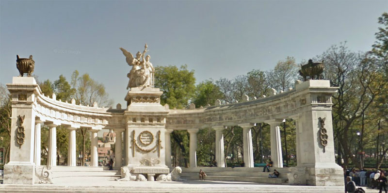
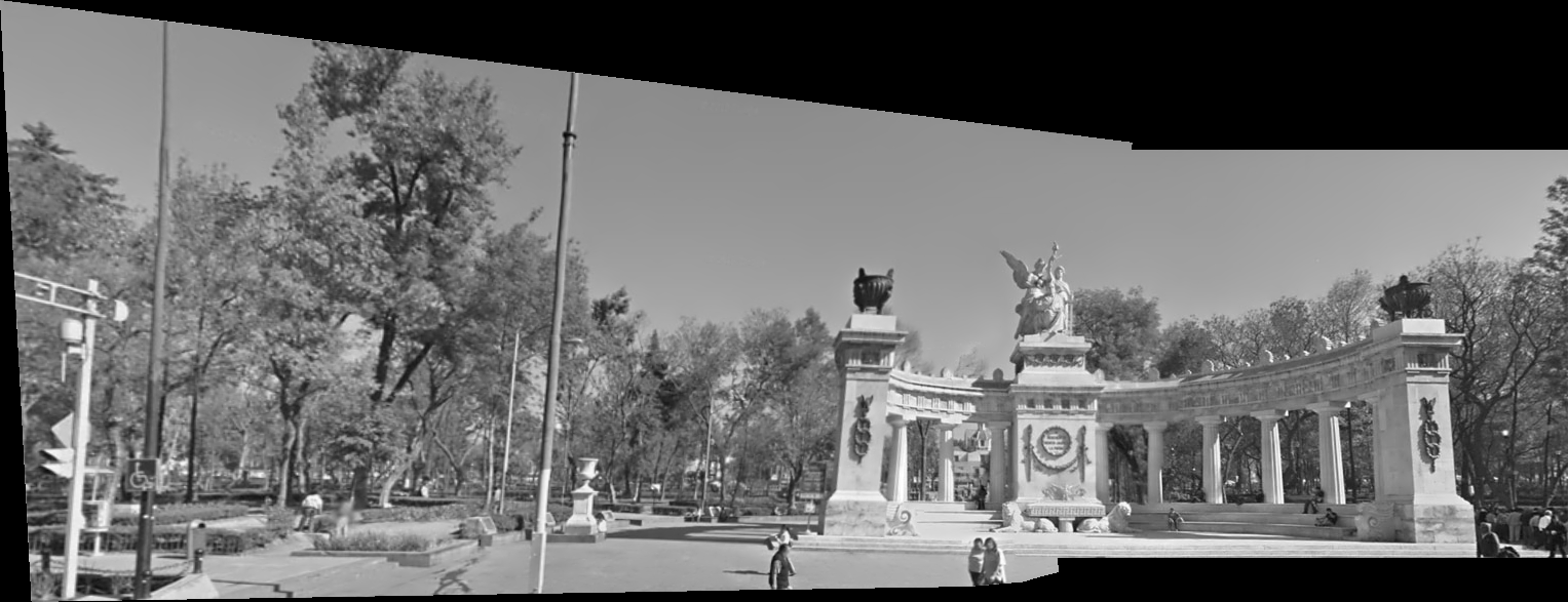
• Experiment with registering very "difficult" image pairs or sequences -- for instance, try to find a modern and a historical view of the same location to mimic the kinds of composites found here. Or try to find two views of the same location taken at different times of day, different times of year, etc. Another idea is to try to register images with a lot of repetition, or images separated by an extreme transformation (large rotation, scaling, etc.). To make stitching work for such challenging situations, you may need to experiment with alternative feature detectors and/or descriptors, as well as feature space outlier rejection techniques such as Lowe's ratio test.
  
  
• Try to implement a more complete version of a system for "Recognizing panoramas" -- i.e., a system that can take as input a "pile" of input images (including possible outliers), figure out the subsets that should be stitched together, and then stitch them together. As data for this, either use images you take yourself or combine all the provided input images into one folder (plus, feel free to add outlier images that do not match any of the provided ones).
  
  
• Implement bundle adjustment or global nonlinear optimization to simultaneously refine transformation parameters between all pairs of images.
  
  
• Learn about and experiment with image blending techniques and panorama mapping techniques (cylindrical or spherical).
  
  

Submission Instructions

You must upload the following files on Canvas:

1. Your code for part 1. The filename should be lastname_firstname_a3_p1.py. We prefer that you upload .py python files, but if you use a Python notebook, make sure you upload both the original .ipynb file and an exported PDF of the notebook.
2. A report in a single PDF file with all your results and discussion for following this template. The filename should be lastname_firstname_a3.pdf.
3. All your output images and visualizations in a single zip file. The filename should be lastname_firstname_a3.zip. Note that this zip file is for backup documentation only, in case we cannot see the images in your PDF report clearly enough. You will not receive credit for any output images that are part of the zip file but are not shown (in some form) in the report PDF.

Please refer to course policies on academic honesty, collaboration, late days, etc.