Fall 2022 CS543/ECE549

Assignment 3: Homography stitching, shape from shading

Due date: Mon, October 30, 11:59:59 PM

Contents

Part 1: Stitching pairs of images

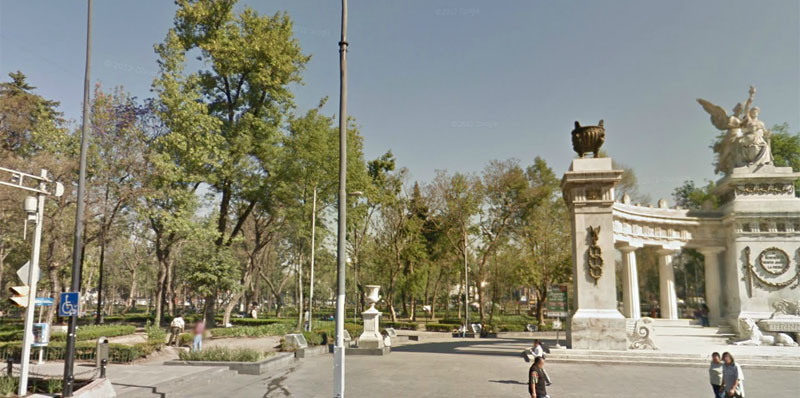
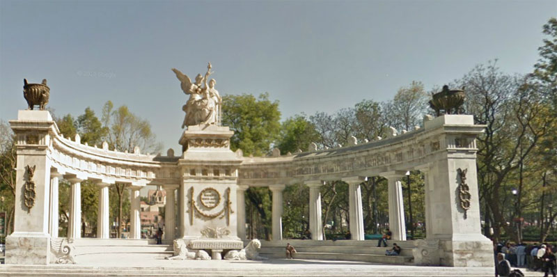
The first step is to write code to stitch together a single pair of images. For this part, you will be working with the following pair (click on the images to download the high-resolution versions):


  1. Download the starter code.

  2. Load both images, convert to double and to grayscale.

  3. Detect feature points in both images. You can use this Harris detector code (it is also copied into the starter .py file), or feel free to use the blob detector you wrote for Assignment 2.

  4. Extract local neighborhoods around every keypoint in both images, and form descriptors simply by "flattening" the pixel values in each neighborhood to one-dimensional vectors. Experiment with different neighborhood sizes to see which one works the best. If you're using your Laplacian detector, use the detected feature scales to define the neighborhood scales.

    Alternatively, feel free to experiment with SIFT descriptors. You can use the OpenCV library to extract keypoints and compute descriptors through the function cv2.SIFT_create().detectAndCompute. This tutorial provides details about using SIFT in OpenCV.

  5. Compute distances between every descriptor in one image and every descriptor in the other image. In Python, you can use scipy.spatial.distance.cdist(X,Y,'sqeuclidean') for fast computation of Euclidean distance. If you are not using SIFT descriptors, you should experiment with computing normalized correlation, or Euclidean distance after normalizing all descriptors to have zero mean and unit standard deviation.

  6. Select putative matches based on the matrix of pairwise descriptor distances obtained above. You can select all pairs whose descriptor distances are below a specified threshold, or select the top few hundred descriptor pairs with the smallest pairwise distances.

  7. Implement RANSAC to estimate a homography mapping one image onto the other. Report the number of inliers and the average residual for the inliers (squared distance between the point coordinates in one image and the transformed coordinates of the matching point in the other image). Also, display the locations of inlier matches in both images by using plot_inlier_matches (provided in the starter .ipynb).

    A very simple RANSAC implementation is sufficient. Use four matches to initialize the homography in each iteration. You should output a single transformation that gets the most inliers in the course of all the iterations. For the various RANSAC parameters (number of iterations, inlier threshold), play around with a few "reasonable" values and pick the ones that work best. Refer to the alignment and fitting lectures for details on RANSAC.

    Homography fitting, as described in the alignment lecture, calls for homogeneous least squares to start a numerical optimizer. The solution to the homogeneous least squares system AX=0 is obtained from the SVD of A by the singular vector corresponding to the smallest singular value. In Python, U, s, V = numpy.linalg.svd(A) performs the singular value decomposition and V[len(V)-1] gives the smallest singular value. I would use SCIPY's scipy.optimize.minmize(see the manual page) to minimize the error in image coordinates.

  8. Warp one image onto the other using the estimated transformation. In Python, use skimage.transform.ProjectiveTransform and skimage.transform.warp.

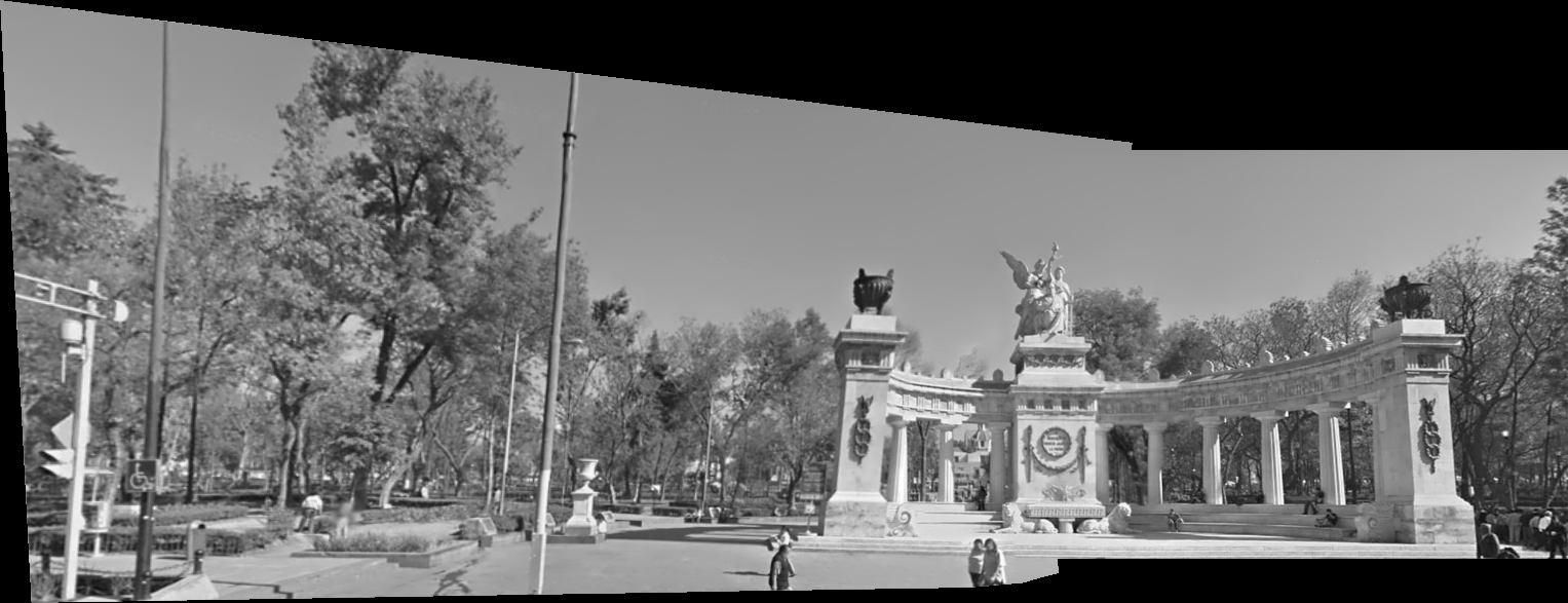
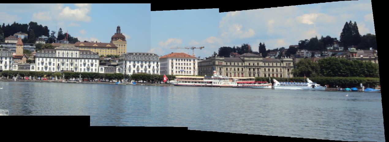
  9. Create a new image big enough to hold the panorama and composite the two images into it. You can composite by averaging the pixel values where the two images overlap, or by using the pixel values from one of the images. Your result should look something like this:


  10. You should create a color panorama by applying the same compositing step to each of the color channels separately (for estimating the transformation, it is sufficient to use grayscale images).

For extra credit

Part 2: Shape from shading


The goal of this part is to implement shape from shading as described in the lecture on light (see also Section 2.2.4 of Forsyth & Ponce 2nd edition).
  1. Download the data and starter code. The data consists of 64 images each of four subjects from the Yale Face database. The light source directions are encoded in the file names. We have provided utilities to load the input data and display the output. Your task will be to implement the functions preprocess, photometric_stereo and get_surface in the ipython notebook, as explained below.

  2. For each subject (subdirectory in croppedyale), read in the images and light source directions. The function LoadFaceImages returns the images for the 64 light source directions and an ambient image (i.e., image taken with all the light sources turned off). The LoadFaceImages function is completed and provided to you in the starter code.

  3. Preprocess the data: subtract the ambient image from each image in the light source stack, set any negative values to zero, rescale the resulting intensities to between 0 and 1 (they are originally between 0 and 255). Complete the preprocess function.

  4. Estimate the albedo and surface normals. For this, you need to fill in code in photometric_stereo, which is a function taking as input the image stack corresponding to the different light source directions and the matrix of the light source directions, and returning an albedo image and surface normal estimates. The latter should be stored in a three-dimensional matrix. That is, if your original image dimensions are h x w, the surface normal matrix should be h x w x 3, where the third dimension corresponds to the x-, y-, and z-components of the normals. To solve for the albedo and the normals, you will need to set up a linear system. To get the least-squares solution of a linear system, use numpy.linalg.lstsq function. Complete the photometric_stereo function.

  5. If you directly implement the formulation from the lecture, you will have to loop over every image pixel and separately solve a linear system in each iteration. There is a way to get all the solutions at once by stacking the unknown g vectors for every pixel into a 3 x npix matrix and getting all the solutions with a single call to numpy solver.

    You will most likely need to reshape your data in various ways before and after solving the linear system. Useful numpy functions for this include reshape, expand_dims and stack.

  6. Compute the surface height map by integration. More precisely, instead of continuous integration of the partial derivatives over a path, you will simply be summing their discrete values. Your code implementing the integration should go in the get_surface function. As stated in the slide, to get the best results, you should compute integrals over multiple paths and average the results. Complete the get_surface function.

    You should implement the following variants of integration:
    1. Integrating first the rows, then the columns. That is, your path first goes along the same row as the pixel along the top, and then goes vertically down to the pixel. It is possible to implement this without nested loops using the cumsum function.
    2. Integrating first along the columns, then the rows.
    3. Average of the first two options.
    4. Average of multiple random paths. For this, it is fine to use nested loops. You should determine the number of paths experimentally.

  7. Display the results using functions display_output and plot_surface_normals included in the notebook.

Extra Credit

On this assignment, there are not too many opportunities for "easy" extra credit. This said, here are some ideas for exploration: If you complete any work for extra credit, be sure to clearly mark that work in your report.

Grading checklist

Part 1: Homography estimation

  1. Describe your solution, including any interesting parameters or implementation choices for feature extraction, putative matching, RANSAC, etc.
  2. For the image pair provided, report the number of homography inliers and the average residual for the inliers (squared distance between the point coordinates in one image and the transformed coordinates of the matching point in the other image). Also, display the locations of inlier matches in both images.
  3. Display the final result of your stitching.

Part 2: Shape from shading

  1. Briefly describe your implemented solution, focusing especially on the more "non-trivial" or interesting parts of the solution. What implementation choices did you make, and how did they affect the quality of the result and the speed of computation? What are some artifacts and/or limitations of your implementation, and what are possible reasons for them?

  2. Discuss the differences between the different integration methods you have implemented for #5 above. Specifically, you should choose one subject, display the outputs for all of a-d (be sure to choose viewpoints that make the differences especially visible), and discuss which method produces the best results and why. You should also compare the running times of the different approaches. For the remaining subjects (see below), it is sufficient to simply show the output of your best method, and it is not necessary to give running times.

  3. For every subject, display your estimated albedo maps and screenshots of height maps (use display_output and plot_surface_normals). When inserting results images into your report, you should resize/compress them appropriately to keep the file size manageable -- but make sure that the correctness and quality of your output can be clearly and easily judged. For the 3D screenshots, be sure to choose a viewpoint that makes the structure as clear as possible (and/or feel free to include screenshots from multiple viewpoints). You will not receive credit for any results you have obtained, but failed to include directly in the report PDF file.

  4. Discuss how the Yale Face data violate the assumptions of the shape-from-shading method covered in the slides. What features of the data can contribute to errors in the results? Feel free to include specific input images to illustrate your points. Choose one subject and attempt to select a subset of all viewpoints that better match the assumptions of the method. Show your results for that subset and discuss whether you were able to get any improvement over a reconstruction computed from all the viewpoints.

Submission Instructions

You must upload the following files on Canvas:

  1. Your code in two separate files for part 1 and part 2. The filenames should be lastname_firstname_a3_p1.py and lastname_firstname_a3_p2.py. We prefer that you upload .py python files, but if you use a Python notebook, make sure you upload both the original .ipynb file and an exported PDF of the notebook.
  2. A report in a single PDF file with all your results and discussion for both parts following this template. The filename should be lastname_firstname_a3.pdf.
  3. All your output images and visualizations in a single zip file. The filename should be lastname_firstname_a3.zip. Note that this zip file is for backup documentation only, in case we cannot see the images in your PDF report clearly enough. You will not receive credit for any output images that are part of the zip file but are not shown (in some form) in the report PDF.

Please refer to course policies on academic honesty, collaboration, late days, etc.